4. Visualización de datos#
La visualización de datos es la representación gráfica de información y datos para facilitar la comprensión, análisis y toma de decisiones.
Facilitar la comprensión: Simplificar datos complejos para que sean comprensibles de un vistazo.
Identificar patrones y tendencias: Destacar relaciones y estructuras en los datos.
Tomar decisiones informadas: Proporcionar una base visual para decisiones fundamentadas.
Comunicar información de manera efectiva: Transmitir mensajes clave de manera clara y concisa.
Caso contrario:

Tomado de: Analytics Vidhya
Otra forma de verlo, es que la visualización de datos es una forma de comprimir datos para que quepan en la memoria humana.
Pero… ya habíamos visto formas de comprimir datos para nuestro entendimiento. ¿Recuerdas cuáles?
Para ejemplificar éste punto, veamos dos ejemplos interesante.
import pandas as pd
import numpy as np
import matplotlib.pyplot as plt
import seaborn as sns
# import plotly.express as px
sns.set()
# Anscombe's quartet
# https://matplotlib.org/stable/gallery/specialty_plots/anscombe.html
x = [10, 8, 13, 9, 11, 14, 6, 4, 12, 7, 5]
y1 = [8.04, 6.95, 7.58, 8.81, 8.33, 9.96, 7.24, 4.26, 10.84, 4.82, 5.68]
y2 = [9.14, 8.14, 8.74, 8.77, 9.26, 8.10, 6.13, 3.10, 9.13, 7.26, 4.74]
y3 = [7.46, 6.77, 12.74, 7.11, 7.81, 8.84, 6.08, 5.39, 8.15, 6.42, 5.73]
x4 = [8, 8, 8, 8, 8, 8, 8, 19, 8, 8, 8]
y4 = [6.58, 5.76, 7.71, 8.84, 8.47, 7.04, 5.25, 12.50, 5.56, 7.91, 6.89]
G = ['I']*11 + ['II']*11 + ['III']*11 + ['IV']*11
X = x*3 + x4
Y = y1 + y2 + y3 + y4
df = pd.DataFrame({'grupo': G, 'x': X, 'y': Y})
df
| grupo | x | y | |
|---|---|---|---|
| 0 | I | 10 | 8.04 |
| 1 | I | 8 | 6.95 |
| 2 | I | 13 | 7.58 |
| 3 | I | 9 | 8.81 |
| 4 | I | 11 | 8.33 |
| 5 | I | 14 | 9.96 |
| 6 | I | 6 | 7.24 |
| 7 | I | 4 | 4.26 |
| 8 | I | 12 | 10.84 |
| 9 | I | 7 | 4.82 |
| 10 | I | 5 | 5.68 |
| 11 | II | 10 | 9.14 |
| 12 | II | 8 | 8.14 |
| 13 | II | 13 | 8.74 |
| 14 | II | 9 | 8.77 |
| 15 | II | 11 | 9.26 |
| 16 | II | 14 | 8.10 |
| 17 | II | 6 | 6.13 |
| 18 | II | 4 | 3.10 |
| 19 | II | 12 | 9.13 |
| 20 | II | 7 | 7.26 |
| 21 | II | 5 | 4.74 |
| 22 | III | 10 | 7.46 |
| 23 | III | 8 | 6.77 |
| 24 | III | 13 | 12.74 |
| 25 | III | 9 | 7.11 |
| 26 | III | 11 | 7.81 |
| 27 | III | 14 | 8.84 |
| 28 | III | 6 | 6.08 |
| 29 | III | 4 | 5.39 |
| 30 | III | 12 | 8.15 |
| 31 | III | 7 | 6.42 |
| 32 | III | 5 | 5.73 |
| 33 | IV | 8 | 6.58 |
| 34 | IV | 8 | 5.76 |
| 35 | IV | 8 | 7.71 |
| 36 | IV | 8 | 8.84 |
| 37 | IV | 8 | 8.47 |
| 38 | IV | 8 | 7.04 |
| 39 | IV | 8 | 5.25 |
| 40 | IV | 19 | 12.50 |
| 41 | IV | 8 | 5.56 |
| 42 | IV | 8 | 7.91 |
| 43 | IV | 8 | 6.89 |
filas = ['grupo']
valores = ['x', 'y']
aggfunc = ['mean', 'std']
df.pivot_table(index=filas, values=valores, aggfunc=aggfunc).round(2)
| mean | std | |||
|---|---|---|---|---|
| x | y | x | y | |
| grupo | ||||
| I | 9.0 | 7.5 | 3.32 | 2.03 |
| II | 9.0 | 7.5 | 3.32 | 2.03 |
| III | 9.0 | 7.5 | 3.32 | 2.03 |
| IV | 9.0 | 7.5 | 3.32 | 2.03 |
Por lo tanto ¿Concluimos que la data del los sets I, II, III y IV son iguales?
# visualice df by grupo in diferent scatter plots
fig, ax = plt.subplots(2, 2, figsize=(6, 6), sharex=True, sharey=True)
ax[0, 0].scatter(x, y1)
ax[0, 0].set_title('Grupo I')
ax[0, 1].scatter(x, y2)
ax[0, 1].set_title('Grupo II')
ax[1, 0].scatter(x, y3)
ax[1, 0].set_title('Grupo III')
ax[1, 1].scatter(x4, y4)
ax[1, 1].set_title('Grupo IV')
fig.tight_layout()
plt.xlim(0, 20)
plt.ylim(0, 14)
plt.show()
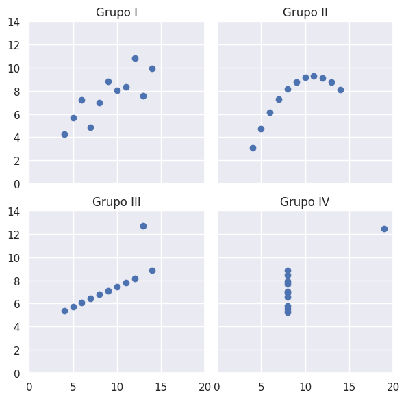
¿Conclusión?
Vamos otro ejemplo.
np.random.seed(123)
# create a bimodal random data
x1 = np.concatenate([np.random.normal(0, 1, 10000), np.random.normal(3, 1, 10000)])
x2 = np.random.normal(x1.mean(), x1.std(), 20000)
data = [[x1.mean(), x1.std()], [x2.mean(), x2.std()]]
pd.DataFrame(data, index=['x1', 'x2'], columns=['mean', 'std']).round(2)
| mean | std | |
|---|---|---|
| x1 | 1.51 | 1.8 |
| x2 | 1.52 | 1.8 |
¿Son iguales?
Ejemplo dataset#
Vamos a trabajar con datos de:
https://www.kaggle.com/datasets/dansbecker/melbourne-housing-snapshot
df = pd.read_csv('https://raw.githubusercontent.com/alejo-acosta/pmdb-material/master/data/melb_data.csv')
df.head()
| Suburb | Address | Rooms | Type | Price | Method | SellerG | Date | Distance | Postcode | ... | Bathroom | Car | Landsize | BuildingArea | YearBuilt | CouncilArea | Lattitude | Longtitude | Regionname | Propertycount | |
|---|---|---|---|---|---|---|---|---|---|---|---|---|---|---|---|---|---|---|---|---|---|
| 0 | Abbotsford | 85 Turner St | 2 | h | 1480000.0 | S | Biggin | 3/12/2016 | 2.5 | 3067.0 | ... | 1.0 | 1.0 | 202.0 | NaN | NaN | Yarra | -37.7996 | 144.9984 | Northern Metropolitan | 4019.0 |
| 1 | Abbotsford | 25 Bloomburg St | 2 | h | 1035000.0 | S | Biggin | 4/02/2016 | 2.5 | 3067.0 | ... | 1.0 | 0.0 | 156.0 | 79.0 | 1900.0 | Yarra | -37.8079 | 144.9934 | Northern Metropolitan | 4019.0 |
| 2 | Abbotsford | 5 Charles St | 3 | h | 1465000.0 | SP | Biggin | 4/03/2017 | 2.5 | 3067.0 | ... | 2.0 | 0.0 | 134.0 | 150.0 | 1900.0 | Yarra | -37.8093 | 144.9944 | Northern Metropolitan | 4019.0 |
| 3 | Abbotsford | 40 Federation La | 3 | h | 850000.0 | PI | Biggin | 4/03/2017 | 2.5 | 3067.0 | ... | 2.0 | 1.0 | 94.0 | NaN | NaN | Yarra | -37.7969 | 144.9969 | Northern Metropolitan | 4019.0 |
| 4 | Abbotsford | 55a Park St | 4 | h | 1600000.0 | VB | Nelson | 4/06/2016 | 2.5 | 3067.0 | ... | 1.0 | 2.0 | 120.0 | 142.0 | 2014.0 | Yarra | -37.8072 | 144.9941 | Northern Metropolitan | 4019.0 |
5 rows × 21 columns
df.info()
<class 'pandas.core.frame.DataFrame'>
RangeIndex: 13580 entries, 0 to 13579
Data columns (total 21 columns):
# Column Non-Null Count Dtype
--- ------ -------------- -----
0 Suburb 13580 non-null object
1 Address 13580 non-null object
2 Rooms 13580 non-null int64
3 Type 13580 non-null object
4 Price 13580 non-null float64
5 Method 13580 non-null object
6 SellerG 13580 non-null object
7 Date 13580 non-null object
8 Distance 13580 non-null float64
9 Postcode 13580 non-null float64
10 Bedroom2 13580 non-null float64
11 Bathroom 13580 non-null float64
12 Car 13518 non-null float64
13 Landsize 13580 non-null float64
14 BuildingArea 7130 non-null float64
15 YearBuilt 8205 non-null float64
16 CouncilArea 12211 non-null object
17 Lattitude 13580 non-null float64
18 Longtitude 13580 non-null float64
19 Regionname 13580 non-null object
20 Propertycount 13580 non-null float64
dtypes: float64(12), int64(1), object(8)
memory usage: 2.2+ MB
df.describe().round(2)
| Rooms | Price | Distance | Postcode | Bedroom2 | Bathroom | Car | Landsize | BuildingArea | YearBuilt | Lattitude | Longtitude | Propertycount | |
|---|---|---|---|---|---|---|---|---|---|---|---|---|---|
| count | 13580.00 | 13580.00 | 13580.00 | 13580.00 | 13580.00 | 13580.00 | 13518.00 | 13580.00 | 7130.00 | 8205.00 | 13580.00 | 13580.00 | 13580.00 |
| mean | 2.94 | 1075684.08 | 10.14 | 3105.30 | 2.91 | 1.53 | 1.61 | 558.42 | 151.97 | 1964.68 | -37.81 | 145.00 | 7454.42 |
| std | 0.96 | 639310.72 | 5.87 | 90.68 | 0.97 | 0.69 | 0.96 | 3990.67 | 541.01 | 37.27 | 0.08 | 0.10 | 4378.58 |
| min | 1.00 | 85000.00 | 0.00 | 3000.00 | 0.00 | 0.00 | 0.00 | 0.00 | 0.00 | 1196.00 | -38.18 | 144.43 | 249.00 |
| 25% | 2.00 | 650000.00 | 6.10 | 3044.00 | 2.00 | 1.00 | 1.00 | 177.00 | 93.00 | 1940.00 | -37.86 | 144.93 | 4380.00 |
| 50% | 3.00 | 903000.00 | 9.20 | 3084.00 | 3.00 | 1.00 | 2.00 | 440.00 | 126.00 | 1970.00 | -37.80 | 145.00 | 6555.00 |
| 75% | 3.00 | 1330000.00 | 13.00 | 3148.00 | 3.00 | 2.00 | 2.00 | 651.00 | 174.00 | 1999.00 | -37.76 | 145.06 | 10331.00 |
| max | 10.00 | 9000000.00 | 48.10 | 3977.00 | 20.00 | 8.00 | 10.00 | 433014.00 | 44515.00 | 2018.00 | -37.41 | 145.53 | 21650.00 |
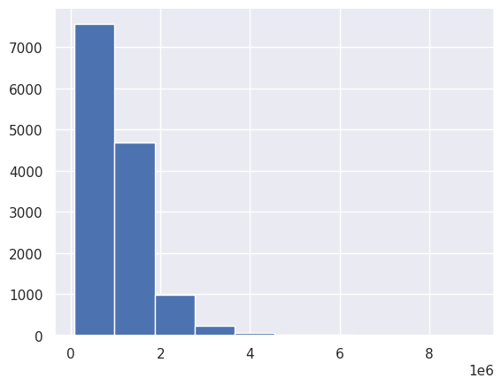
df['Price'].hist()
<Axes: >
lista = ['CHUQUIMARCA/ARGUELLO DANIELA NICOLE','FREIRE/VARGAS MELANY BELÉN','GUAMAN/TIPAN JUAN FRANCISCO','PAREDES/ERAZO MARÍA JOSÉ','GONZALEZ/MENDEZ ARIAN MARCELO','PANCHANA/COTO STEPHANO ALBERTO','RAMIREZ/NAVARRO MARTIN RICARDO','VASCONEZ/CELI GABRIELA VIVIANA','VERDEZOTO/BARBA EVELYN ADRIANA','ANAGUANO/PERALVO ALAN ARIEL','DAVILA/JIMENEZ CAROLINA ESTEFANIA','TERAN/TOSCANO STEFANO MATEO','CHICAIZA/JAGUACO BRAYAN JAIR','CARTAGENOVA/ECHEVERRIA ISAAC ','GONZALEZ/MENDEZ ARIEL MARTIN','MORALES/VELEZ DILAN ALEJANDRO','PILLIGUA/PEÑAHERRERA FRANCISCO XAVIER',]
np.random.choice(lista, 1)[0]
np.str_('TERAN/TOSCANO STEFANO MATEO')
Gráficos interactivos - Plotly#
import plotly.express as px
gapminder = px.data.gapminder()
tips = px.data.tips()
px.box(tips,x = 'day',y='total_bill', title= 'Boxplot por dia con dias en orden', category_orders= {'day': ["Thur","Fri","Sat", "Sun"]})
px.scatter(gapminder, x="gdpPercap", y="lifeExp",
animation_frame="year", animation_group="country",
size="pop", color="continent", hover_name="country",
log_x=True, size_max=45, range_x=[100,100000], range_y=[25,90])
px.scatter(gapminder, x="gdpPercap", y="lifeExp",
animation_frame="year", animation_group="country",
size="pop", color="continent", hover_name="country",
facet_col="continent",
log_x=True, size_max=30, range_x=[100, 100000], range_y=[25, 90])